EM algorithm to impute missing value and underlying parameter

 Genetic linkage data are from Rao, C. R. (1973), Linear Statistical Inference and Its Applications, 2nd Ed., New York: John Wiley & Sons. p368


x<-c(125,18,20,34)
n<-sum(x)
theta.0<-(x[1]-x[2]-x[3]+x[4])/n
theta.0
current_theta<-c()
new_theta<-c()
z11<-c()
z12<-c()
i<-1
current_theta[i]<-theta.0

new_theta[i]<-(x[1]*current_theta[i]+2*x[4]+x[4]*current_theta[i])/(n*current_theta[i]+2*(x[2]+x[3]+x[4]))
new_theta[i]
difference<-abs(new_theta[i]-current_theta[i])
difference

while(difference>0.00000001){
current_theta[i]<-new_theta[i]
new_theta[i+1]<-(x[1]*current_theta[i]+2*x[4]+x[4]*current_theta[i])/(n*current_theta[i]+2*(x[2]+x[3]+x[4]))
difference<-abs(new_theta[i+1]-current_theta[i])
z11[i]<-(0.5/(0.5+0.25*current_theta[i]))*x[1]
z12[i]<-((0.25*current_theta[i])/(0.5+0.25*current_theta[i]))*x[1]
i<-i+1
}
cbind(theta=current_theta,Z11=z11,Z12=z12)

Results: Z11 and Z12 are imputed missing values and thetas are mle estimate of parameter, 7 iterations will get 10^-8 accuracy.


        theta             Z11               Z12
[1,] 0.6251317     95.23332     29.76668
[2,] 0.6265968     95.18019     29.81981
[3,] 0.6267917     95.17314     29.82686
[4,] 0.6268175     95.17220     29.82780
[5,] 0.6268210     95.17207     29.82793
[6,] 0.6268214     95.17206     29.82794
[7,] 0.6268215     95.17206     29.82794

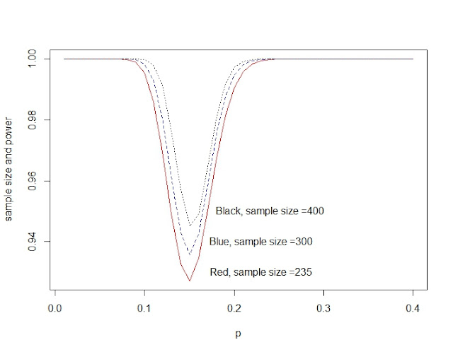
Power and sample size for Binomial distribution

power_n<-function(size){
p0<-51/235 #for calculate the critical region
c<-qbinom(p0,size, 1/6)
p<-seq(0.01,0.4,0.01)
pow<-1-dbinom(c,size,p)+dbinom(size-c,size,p) #the second part is very small can be omitted.
return(pow)
}
p<-seq(0.01,0.4,0.01)
plot(p,power_n(235),type="l",col="red")
lines(p,power_n(300),lty=2,col="blue")
lines(p,power_n(400),lty=3, col="black")
text(0.23,0.93,"Red, sample size =235")
text(0.23,0.94,"Blue, sample size =300")
text(0.24,0.95,"Black, sample size =400")

Rao-Cramer Lower Bound and Efficiency

The most racist places in America

MLE estimates

On 25 February 2015, the journal Basic and Applied Social Psychology issued an editorial banning p -values and confidence intervals from all future papers.

http://www.tandfonline.com/doi/pdf/10.1080/01973533.2015.1012991

Use Newton-Raphson Method to calculate MLE of a Cauchy distribtuion

mlecauchy=function(x,toler=.001){      #x is a vector here
startvalue=median(x)
n=length(x);
thetahatcurr=startvalue;
# Compute first deriviative of log likelihood
firstderivll=2*sum((x-thetahatcurr)/(1+(x-thetahatcurr)^2))
# Continue Newton’s method until the first derivative
# of the likelihood is within toler of 0.001
while(abs(firstderivll)>toler){
# Compute second derivative of log likelihood
secondderivll=2*sum(((x-thetahatcurr)^2-1)/(1+(x-thetahatcurr)^2)^2);
# Newton’s method update of estimate of theta
thetahatnew=thetahatcurr-firstderivll/secondderivll;
thetahatcurr=thetahatnew;
# Compute first derivative of log likelihood
firstderivll=2*sum((x-thetahatcurr)/(1+(x-thetahatcurr)^2))
}
list(thetahat=thetahatcurr);
}
x<-c(-1.94,0.59,-5.98,-0.08,-0.77)
mlecauchy(x,0.0001)

###########result########'
####   $thetahat
####  [1] -0.5343968

#####use the R biuld in funcion ######

optimize(function(theta) -sum(dcauchy(x, location=theta, log=TRUE)), c(-100,100)) #we use negative sign here,
                                                                                  #by default it return a minimum
#optimize(function(theta) sum(dcauchy(x, location=theta, log=TRUE)),maximum=T, c(-100,100))

#########Result###############

###  $minimum
###  [1] -0.5343902
###   $objective
###  [1] 11.2959


Almost the same for the two methods.